
Beyond Data Discovery: What You Can Do with OpenTopography's New Raster STAC
Sep 21, 2026
OpenTopography has deployed a SpatioTemporal Asset Catalog (STAC) catalog for our raster digital elevation model (DEMs) datasets. This allows users to programmatically search, browse, and access our full library of open digital elevation model (DEM) datasets, including global products (e.g., Copernicus DEM) and high-resolution, lidar-derived regional datasets. You can explore the catalog directly in the STAC Browser or connect to it programmatically via the endpoint at https://portal.opentopography.org/stac/raster_catalog.json
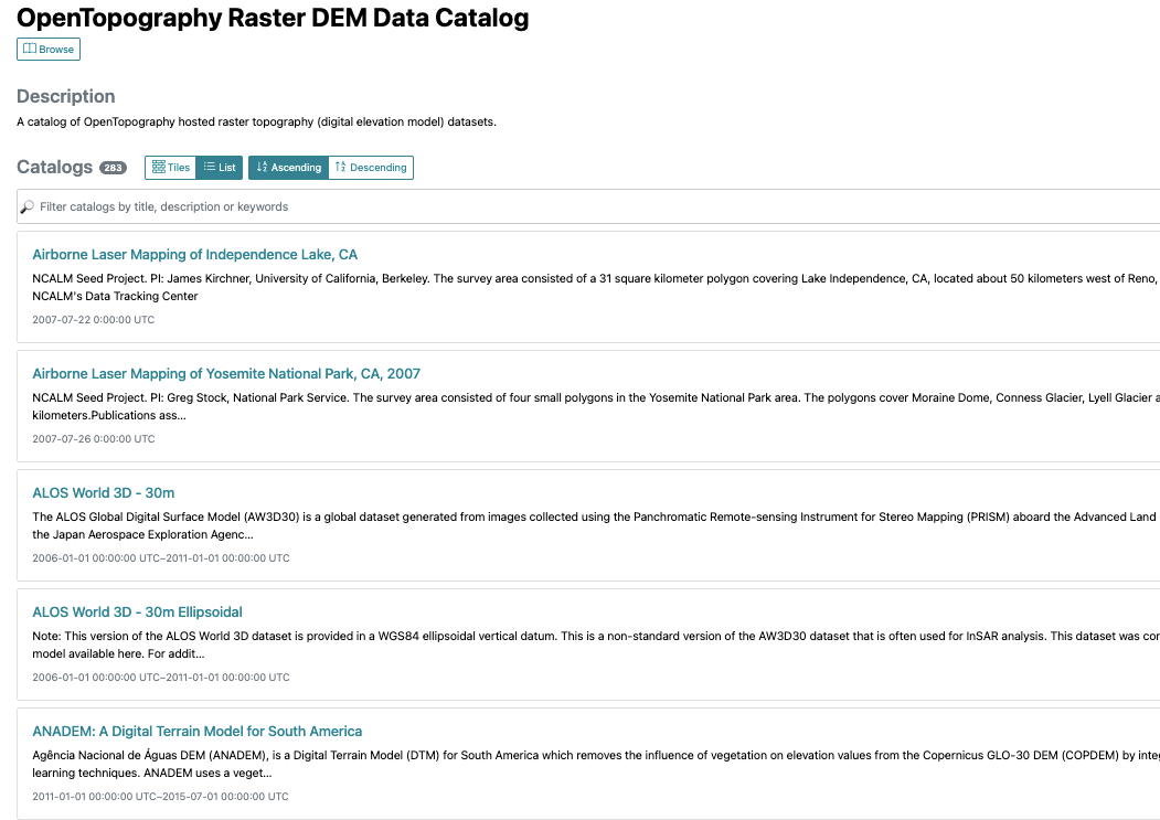
STAC Browser interface showing the data collections.
To highlight what the STAC catalog can do, we created two example Jupyter notebooks that demonstrate how OpenTopography's Raster STAC goes far beyond simple file and metadata search.
A Quick Refresher: What Makes STAC Different
STAC is an open specification for describing geospatial data in a consistent, machine-readable way. Every dataset in our catalog — a "collection" in STAC terms — carries structured metadata: spatial and temporal extent, provider information, licensing, and even a formal DOI and citation string.
One of STAC's biggest advantages is how lightweight it can be compared to more traditional geospatial data catalogs. A STAC catalog doesn't need a heavyweight database system behind it to function — it can be as simple as a set of static JSON files served over plain HTTP, or scaled up into a searchable API. Either way, the same open metadata structure applies, which keeps a STAC catalog easy to host, mirror, and query without sacrificing structure or machine-readability.
Because the metadata follows an open, shared standard, any STAC-aware tool can query it, filter it, and pull assets from it. That interoperability is a genuine strength of the format. But the more interesting story is what becomes possible once you connect to the catalog and start working with the data directly — and that's what the two example notebooks below demonstrate.
Notebook 1: Streaming Data Without Downloading Large Files
Our simple example notebook starts where most workflows do: connecting to the catalog, looping through collections, and finding items that intersect a given bounding box. It then goes beyond data discovery and opens the matching dataset in place, directly from the cloud, and generates a hillshade visualization without downloading the entire file to disk.
This works because OpenTopography's raster assets are stored as Cloud Optimized GeoTIFFs (COGs). Because COGs are internally structured to allow HTTP range requests, applications can stream only the pixels they need. The notebook leverages this capability to read remote elevation values and generate interactive shaded-relief maps in seconds.
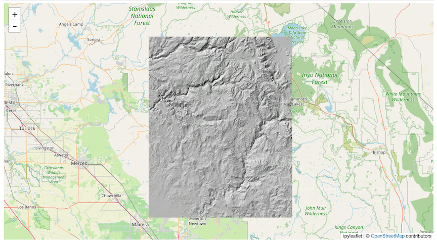
A hillshade overlay rendered on the ipyleaflet map from the Jupyter notebook
Why it matters: for a quick look at terrain - checking whether a dataset actually covers the area you care about, or getting a first visual impression - you no longer need to download numerous files just to find out.
Notebook 2: Point, Click, Explore
The interactive notebook takes this further and turns the whole workflow into a guided, map-first experience. Instead of hardcoding coordinates, you:
- Draw a bounding box directly on a map to define your area of interest.
- Search all collections in parallel, using a thread pool so the query returns in seconds instead of minutes.
- Pick a dataset from a dropdown of everything that intersects your search area.
- Inspect full metadata — including the DOI and citation string — before committing to anything.
- Generate a color terrain hillshade rendered from a memory-safe, downsampled read of the COG (so even huge rasters don't crash your notebook).
- Download the outputs — both the rendered image and the metadata JSON — with one click.
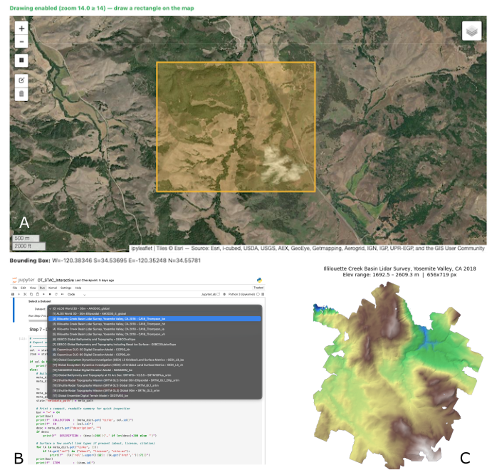
A. Users can select an area on a map from within the notebook. B. A listing of intersecting datasets will populate the drop-down list. C. A colorized hillshade will be created over the area of interest.
Why it matters: this is discovery, visualization, and citation-ready provenance in a single, exploratory loop — no need to already know exactly what dataset or coordinates you want before you start.
The Bigger Picture
Put together, these two notebooks highlight capabilities that go well beyond "find it and download it":
- Cloud-native partial reads — work with a DEM's pixels directly, without downloading the whole file.
- On-the-fly derived products — generate hillshades and other visualizations right in your analysis, from remote data.
- Interactive, map-driven search — explore an area visually instead of hardcoding coordinates.
- Parallelized search at scale — query hundreds of collections at once.
- Built-in provenance — every dataset carries a DOI and citation, ready for reproducible research.
- Standards interoperability — because it's plain STAC, any STAC-aware client or plugin (QGIS, other STAC browsers, your own code) can use OpenTopography's catalog just as easily as ours can.
Try It Yourself
Both notebooks are open source and ready to run in Google Colab — no local setup required:
Or browse the catalog directly at the OpenTopography STAC Browser.